Notebook Title

Authors: Author 1, Author 2, etc.

Keywords: [keywords that describe the content of the notebook, comma separated]

Abstract

[Insert Abstract Here]

Introduction

[Insert Introduction Here]

Methods

[Insert Methods Here]

Math and Equations

Equations can be included in your notebooks by either using $$ symbols to wrap the equation or by using the \begin{equation} to start an equation/math block. Please see the examples below:

Example 1: Using $$

\[ x = \frac{-b \pm \sqrt{b^2 - 4ac}}{2a} \]

You can use LaTeX syntax for equations in your documents. For example, here is an example of a cross-product:

Example 2:

(1)\[\begin{equation} \label{matrix} \mathbf{u} \times \mathbf{v}=\left|\begin{array}{ll}u_{2} & u_{3} \\ v_{2} & v_{3}\end{array}\right| \mathbf{i}+\left|\begin{array}{ll}u_{3} & u_{1} \\ v_{3} & v_{1}\end{array}\right| \mathbf{j}+\left|\begin{array}{ll}u_{1} & u_{2} \\ v_{1} & v_{2}\end{array}\right| \mathbf{k} \end{equation}\]

Using the $$ syntax, one can easily reference the equation too. For example here is the equation 1 with a label added that can be referenced:

(2)\[ x = \frac{-b \pm \sqrt{b^2 - 4ac}}{2a} \]

Referencing and Cross-Referencing

Linking to equations

You can easily link to these equations using {eq}label syntax. For example here is a link to example (2) equation.

Referencing figures

To reference a figure in your notebook, first add the figure with a name. Next use the name to reference it.

🛠 Double click the next cell to see the MyST {figure} syntax.

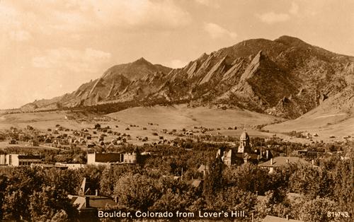
https://artsourceinternational.com/wp-content/uploads/2018/04/P-1984-1.jpg

Fig. 1 My bold mountain 🏔🚠.

Check out how we referenced this figure: My bold mountain 🏔🚠.!!

Referencing Tables

To reference a table, first create a table and give it a name.

Table 1 My table title
Month	Temperature (°C)
January	5
February	6
March	10
April	15
May	20
June	25
July	30
August	30
September	25
October	18
November	10
December	5

Now, you can reference this table My table title!!

Code Block Outputs

Jupyter Book will also embed your code blocks and output in your book. For example, here’s some sample Matplotlib code:

from matplotlib import rcParams, cycler
import matplotlib.pyplot as plt
import numpy as np
plt.ion()

<contextlib.ExitStack at 0x10706d1f0>

# Fixing random state for reproducibility
np.random.seed(19680801)

N = 12  # 12 months
data = [np.logspace(0, 1, 100) + np.random.randn(100) + ii for ii in range(N)]
data = np.array(data).T
monthly_medians = np.median(data, axis=0)


cmap = plt.cm.coolwarm
rcParams['axes.prop_cycle'] = cycler(color=cmap(np.linspace(0, 1, N)))


from matplotlib.lines import Line2D
custom_lines = [Line2D([0], [0], color=cmap(0.), lw=4),
                Line2D([0], [0], color=cmap(.5), lw=4),
                Line2D([0], [0], color=cmap(1.), lw=4)]

fig, ax = plt.subplots(figsize=(10, 5))
lines = ax.plot(data)
ax.legend(custom_lines, ['Cold', 'Medium', 'Hot']);

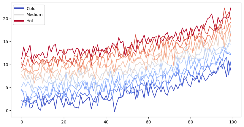
Note that the image above is captured and displayed in the published paper.

Discussion

[Insert Discussion Here]

Conclusion:

[Insert Conclusion Here]

References

Using the following syntax will automatically create the bibliography from the references.bib file.

```{bibliography}
```

PGH11: Fernando Perez, Brian E Granger, and John D Hunter. Python: an ecosystem for scientific computing. Computing in Science \\& Engineering, 13(2):13–21, 2011.